You became an SEO to help people grow great businesses. No one said anything about spending hours dealing with Excel data.
The bigger the web becomes the more data there is that needs processing.
Excel contains a huge number of standard formulas. A reference guide to these should be your first step to speeding up your Excel number crunching. There are also great tools like SEO Tools For Excel that deal with SEO specific issues.
But what if using them is very repetitive or they don’t quite do what you are looking for? Wouldn’t it be great if you could automate a whole series of tasks?
If there’s something that you do often in Excel (for example, weekly reports) that requires you to carry out a series of tasks repetitively then an Excel macro is what you need. It will let you record the steps that you go through once and then, at the click of a button, apply them to any spreadsheet.
A simple example would be formatting weekly data that you are sent so that you can upload it to a website (product information, event dates etc).
You can guarantee that the data won’t come in the format required by your CMS. The dates won’t be in the correct format, the columns won’t be in the right order, financial information will have a dollar sign where it’s not needed or vice-versa. All of which you have to fix by hand each time.
A well written macro will take all of this aggravation away. Push a button and the data is in the format required, upload it to your CMS and you’re done. The more repetitive the task the better a macro is suited to it.
Great so how do I create a macro?
Let’s split this into 5 sections:
- What Is A Macro?
- How Do I Create A Macro?
- How Do I Run My Macro
- Adding Your Most Used Macros To Your Excel Toolbar
- A Couple Of Things To Beware Of

1. What Is An Excel Macro?
Think of an Excel spreadsheet as the HTML in a web page and the Excel macro which manipulates the spreadsheet as the jQuery that you use to manipulate the HTML.
To create jQuery you need to be a coder. The best bit about macros is that anyone can write them. You simply physically show Excel the actions that you would like it to carry out and Excel writes the code for you.
Remember Excel will copy what you do exactly. It’s worth taking a couple of minutes before creating a macro to plan things out.
2. How Do I Create A Macro in Excel?
For this example I’ve used a very short GA download.
- Click the “View” tab. This will bring up the Workbook ribbon.
- Click the “Macros” button in the macros group. This is usually on the far right of the ribbon. This will bring up a drop down menu.
- Click “Record Macro….”
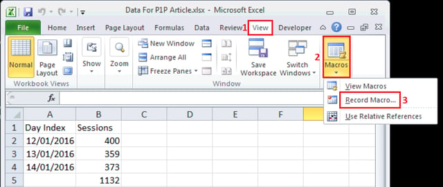
You will now be presented with the “Record Macro” dialogue box.
This asks for 4 inputs.
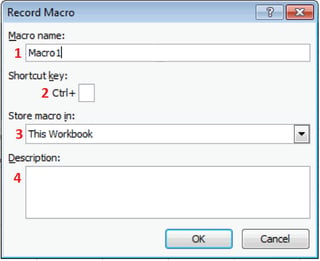
1: “Macro name:”
Do take 10 seconds to think of a clear name. By next week the Excel generated name of “Macro1” won’t be very helpful. If you use a number of macros to do similar things it’s irritating when you run the wrong one.
Excel does not allow spaces in macro names so people generally use underscore_to_separate_words.
2: “Shortcut key:”
Optional. This allows you to create a shortcut key for your macro which makes running it incredibly quick. The only thing to remember is that you can’t use the same key combination as any of Excel’s existing shortcuts.
3: “Store macro in:”
This asks you where you would like to store your macro.
By default this will show “This Workbook”. This will save the macro to the current workbook. It won’t be available to you in other workbooks if you choose this.
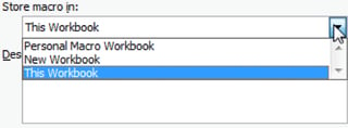
Saving your macro in your “Personal Macro Workbook” will save it to a file called “Personal.xlsm”. This means that your macro will be available whenever you open Excel.
Finally saving in a “New Workbook” creates a new workbook which it will record your macros into.
4: “Description:”
Optional. As with a name, I would recommend that you spend 20 seconds typing in a quick description. This avoids confusing your macros if you have a number.
Having done all of this, click “OK” and you’re off.
Excel will now record everything that you do. You name it, it will record it – creating new workbooks or charts, changing number formatting even down to moving and resizing windows.
If you’re unsure if you’re in record mode there are a couple of ways to tell.
Firstly in the bottom left of your Excel window there will be a small change. A Stop button will have appeared, which you can click to stop recording.

The bottom left of you spreadsheet would usually look as below. The spreadsheet icon is actually a start button for recording a macro which brings up the “Record Macro” dialogue box we discussed above if you click it.

You can now simply record the actions that you would like Excel to carry out.
Once you have completed all of the tasks that you would like to include in your macro click the button in the bottom left of your Excel window to stop recording.
Alternatively you can use the Macro button in your ribbon.
- Click the "Macros" button in the ribbon
- Click "Stop Recording" option
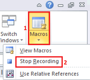
Congratulations. You have successfully recorded your first macro.
3. How Do I Run My Macro?
Running your macro is incredibly simple.
- Click the "Macros" button in your ribbon.
- Click "View Macros"
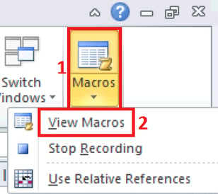
To run a macro you simply:This will bring up the “Macro” dialogue box. This lists all of the macros available to you.
- Select the macro you want from the list.
It will now be highlighted in blue and appear above the list.
- Click "Run"
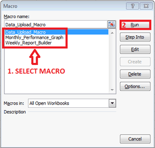
Congratulations you’ve now run your first macro.You can now sit back (briefly!) and enjoy watching your macro do the hard work.
4. Adding Your Most Used Macros To Your Excel Toolbar
Excel offers the option of adding your macro to your Excel toolbar so that you can run it at the click of a button. For frequently used macros this is a handy time saver.
To do this right click anywhere in your Excel ribbon and then choose ‘Customise Quick Access Toolbar….” from the menu that you are now offered.
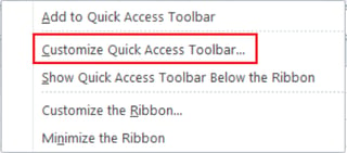
In case you aren’t clear on the difference between the ribbon and the Quick Access Toolbar (‘QAT’) in Excel

You will then be presented with the “Excel Options” dialogue box, as below, which is a little confusing.
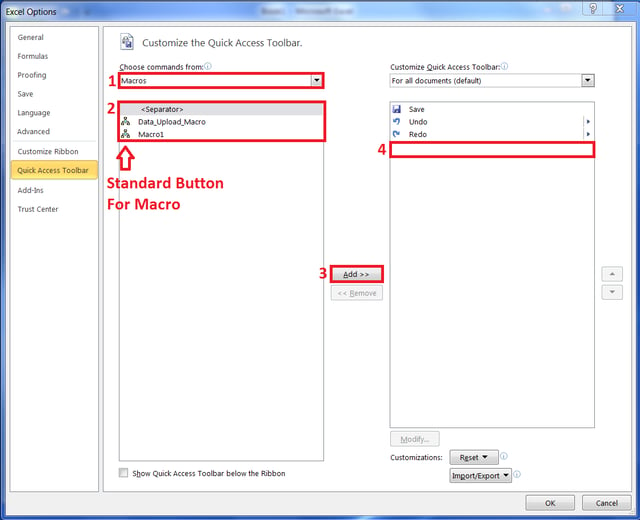
Let’s take this step-by-step.
- Click on the “Choose commands from:” dropdown menu. Choose “Macro” from the list of options. It will be third probably.
Note: I have already clicked on macro in this screenshot. Initially the dropdown menu box will contain “Popular Commands”.
- Click on the macro that you would like to add to your QAT from the list below.
- Click on the “Add” button
- Your macro should now appear where box 4 is, in the right-hand column.
The small icon to the left of your macro is the icon that the button for your macro will contain by default.
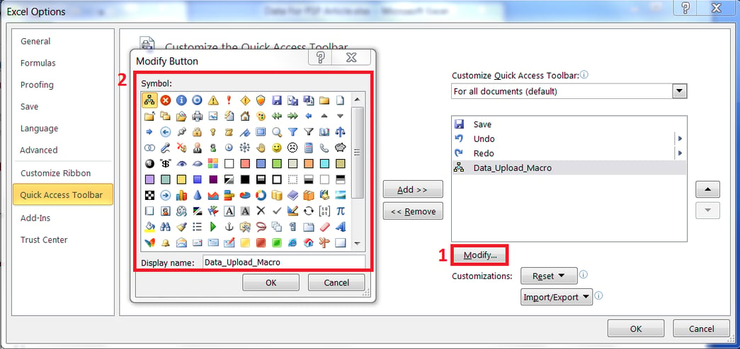
If you would like to customize this click the “Modify…” button below your macro.
Excel then presents you with the “Modify Button” dialogue box.
The second step is to then to choose the icon that you would like to use for this button by clicking on it. Finally, click “OK” below the icons to confirm your choice.
The icon to the left of your macro should now have changed. To complete this entire process, click “OK” in the “Excel Options” dialogue box.
You have now added the button to your QAT. For this example I have chosen a chequered flag.

5. A Few Notes: Relative References & Security
- Relative References
As I said earlier in the article Excel records exactly what you do. So if you click on cell B3 when recording your macro when you run your macro it will always choose cell B3. This is known as absolute referencing and is the default setting.
What if you would like it to choose a cell relative to the one that you have highlighted when you run your macro? For example, you want it to apply certain formatting to the cell that you are in and the two cells to the left of the one that you are in, wherever you are in your spreadsheet.
This requires you to turn on relative referencing.
To do this, simply open the “Macros” menu and the third choice down is “Use Relative Referencing”. Click this and then record your macro to use relative references.
As per the example below the icon to the left of the menu will now be highlighted.
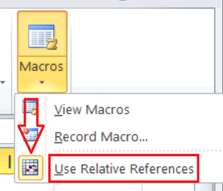
Be careful though. This option will remain turned on until you turn it off. If you are having issues with a macro doing unexpected things this setting is the first thing to double check.
- Security
Macros are very powerful. They can change things beyond the spreadsheet that they sit in. As a consequence they have been used to spread viruses.
If you receive an email with a macro enabled spreadsheet it bears repeating that you should not open it unless it comes from a trusted source.
To learn more about macro security I would recommend Excel Easy.
So there we have it, creating your own macro in Excel. Who knew that Microsoft could be so helpful or save you so much time!
NB: The screen shots in this tutorial are taken from a Windows 7 / Excel 2010 machine. The steps will be unchanged if your set up is different although visually it will probably look a little different.

