To: Linkaratiers
From: Nicholas Chimonas
Welcome to what I hope is an early spring edition of Tutorial Tuesday. In today’s tutorial you will learn how to filter out the noise from large sets of keyword ranking data, and identify meaningful takeaways to help inform your link building & SEO strategy.
Massive data sets that exist as raw Excel sheets are not easy to interpret meaning from, so you need to distill the data down to digestible sizes in order to understand what data is signficant. Today’s half of this process is focused on formatting your data set using a Chimonas approved method, both for the purposes of isolating the important data points, and for ease of use by humans, bosses, and YOU!
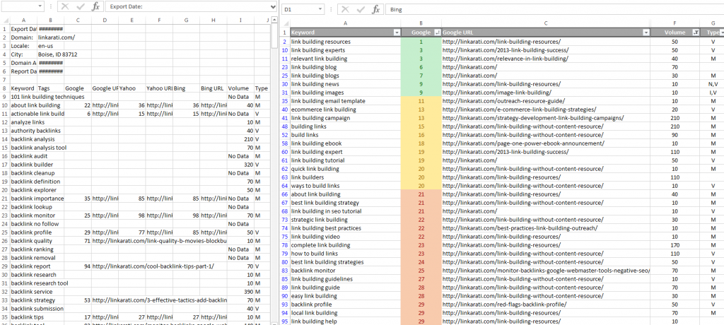
Robots to the left, humans to the right.
The point of this process is to identify keyword ranking opportunities and missed chances. Keep in mind that this is a microscopic viewpoint, and the macroscopic is just as important for other applications. This simple technique can help guide link building and keyword strategy.
This guide begins at the point where you already have large amounts of keyword ranking data, but you’re not sure where to start or how to disseminate meaning behind the numbers.
If you do not already have keyword data, check out Jesse Stoler’s Tutorial Tuesday on using Ubersuggest to discover relevant keywords, so you can plug and play with this tutorial. Then acquire ranking data with your favorite ranking tool. Serplab.co.uk is a good free one, but I’ll be using Authority Labs data for this walk through.
1. Download keyword ranking data as CSV or Excel from your favorite ranking tool.
2. Clean your column header row. Here's how:
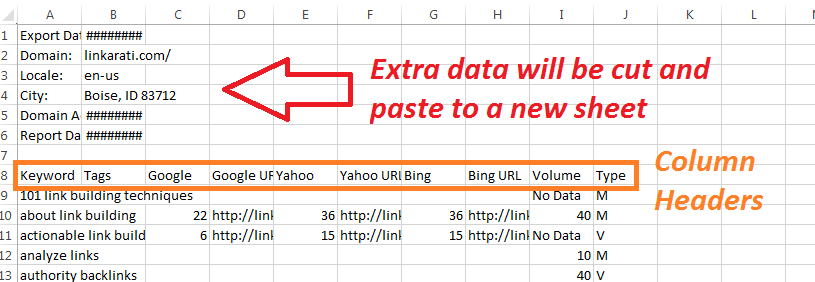
2a. If extra data is above your column headers, move it to a new sheet tab.
2b. Delete any empty rows and columns, and freeze the top row.
- Once you've deleted the empty rows above your column headers so that they are located in row 1, click on the "1" of row 1 to highlight it.
- Click the "View" tab at the top of Excel.
- Click "Freeze Panes".
- Click Freeze Top Row.
- Scroll down and observe the effect of the Excel spell you just invoked! Cool.
2c. Give the header an easy to read color format. Delete or hide unnecessary columns.
- Click the "Home" tab at the top of Excel.
- Click the "Check Cell" box in the "Styles" formatting section of the "Home" top toolbar.
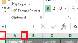
- Click the triangle "select all" button adjacent to row 1 and column A.
- Double click the column divider line between column A and column B to expand all columns.
- Right click any unnecessary columns and select "Hide".
- For the Authority Labs data that I'm working with, I keep keyword data, Google rankings, Bing rankings, search volume, and result type.
- A nice touch is to "center" all data columns besides keywords and URLs.
Follow the red boxes to find your center.
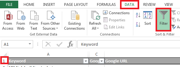
3. Apply a data filter. Organize and Filter your data! [Steps below]
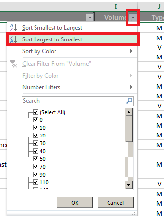
3a. First, sort search volume in descending order.
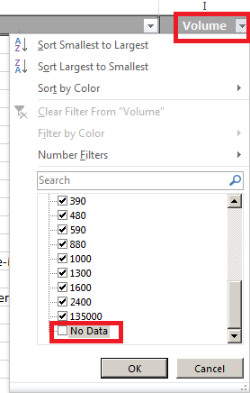
3b. Second, filter out"0", "No Data", and "(blank)" by un-checking their corresponding boxes, so that we only see rankings with registered relative search volume.
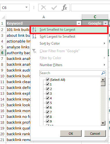
3c. Next, sort rankings in ascending order.
4. Apply a heat map with conditional formatting.
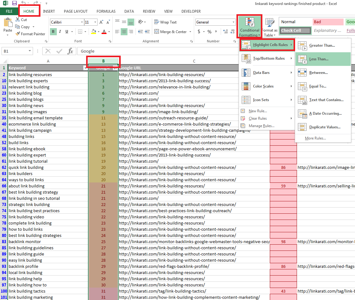
- Navigate to the "Home" tab.
- Highlight your Google rankings column by clicking on the column letter (in my case, column B).
- Click "Conditional Formatting" in the "Styles" section of the "Home" tab.
- Hover your mouse over "Highlight Cell Rules".
4a. Define the conditional formatting rules.
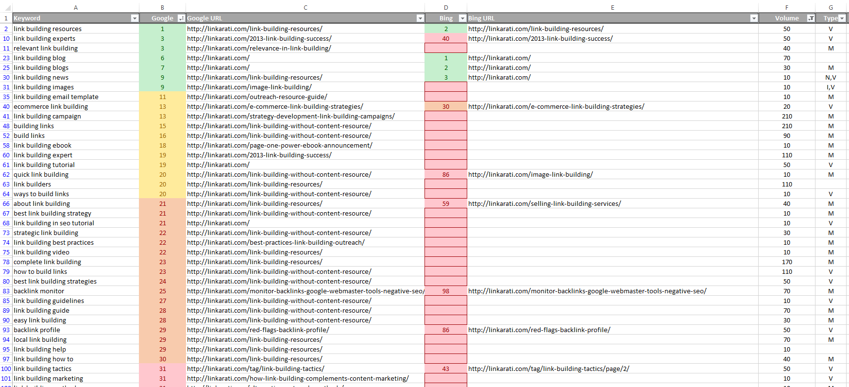
- In order to highlight keywords ranking on page 1, click "Less Than" (see above), enter "11", and select green as the cell fill color.
- For page 2 rankings, click "Between...", enter "11" and "21", and select yellow as the cell fill color.
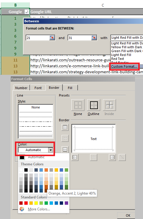
- For page 3 rankings, click "Between...", enter "21" and "31", and select orange as the cell fill color. Pro tip: You'll have to click "custom format", then "color" to get to orange.
- For everything below page 3 rankings, select "Greater than", enter "30", and select red for the cell fill color.
- [Optional] If you're tracking rankings from other search engines in a different column, copy and "special paste" just your formatting to the other ranking data columns.
- Copy the entire column you just applied conditional formatting rules to,
- Right click the column you want to apply the formatting to, and select "Formatting".
5. Enjoy the finished product!
Don't forget to save the spreadsheet as .xlsx (Excel Workbook), DO NOT save as .csv. Otherwise, your formatting will not be saved.
Ah... Now that's easy on the eyes. I don't always look at spreadsheets, but when I do, I drink Tecate. Er, I mean, Dos Equis.
You may remember that at one point we sorted our "Volume" column in descending order. Scroll down the sheet to all of the keywords that do not have registered rankings, and you'll notice that your biggest targets are all sorted by descending volume. This is useful data to help prioritize bigger initiatives.
Now that we have isolated the most important data under a microscopic and aesthetically pleasing view, there are many ways to digest this information to guide your link building and keyword strategy. From here, we want to identify which keywords would be worth focusing on to improve their corresponding page’s ranking. Primarily, your pages that are ranking on search engine result pages 1, 2, and 3 will present the best opportunities for quickly capturing additional traffic.
Tune in next week for another edition of Tutorial Tuesday, where I will guide you through my method of assessing the meaning behind the data to capitalize on new traffic opportunities, and develop strategic takeaways. Happy Excelling!


